Gaussian Assumption for Normality

The Gaussian (normal) distribution is a key assumption in many statistical methods. It is mathematically represented by the probability density function (PDF):

\[f(x) = \frac{1}{\sqrt{2\pi\sigma^2}} \exp\left(-\frac{(x-\mu)^2}{2\sigma^2}\right)\]

where:

• \(\mu\) is the mean

• \(\sigma^2\) is the variance

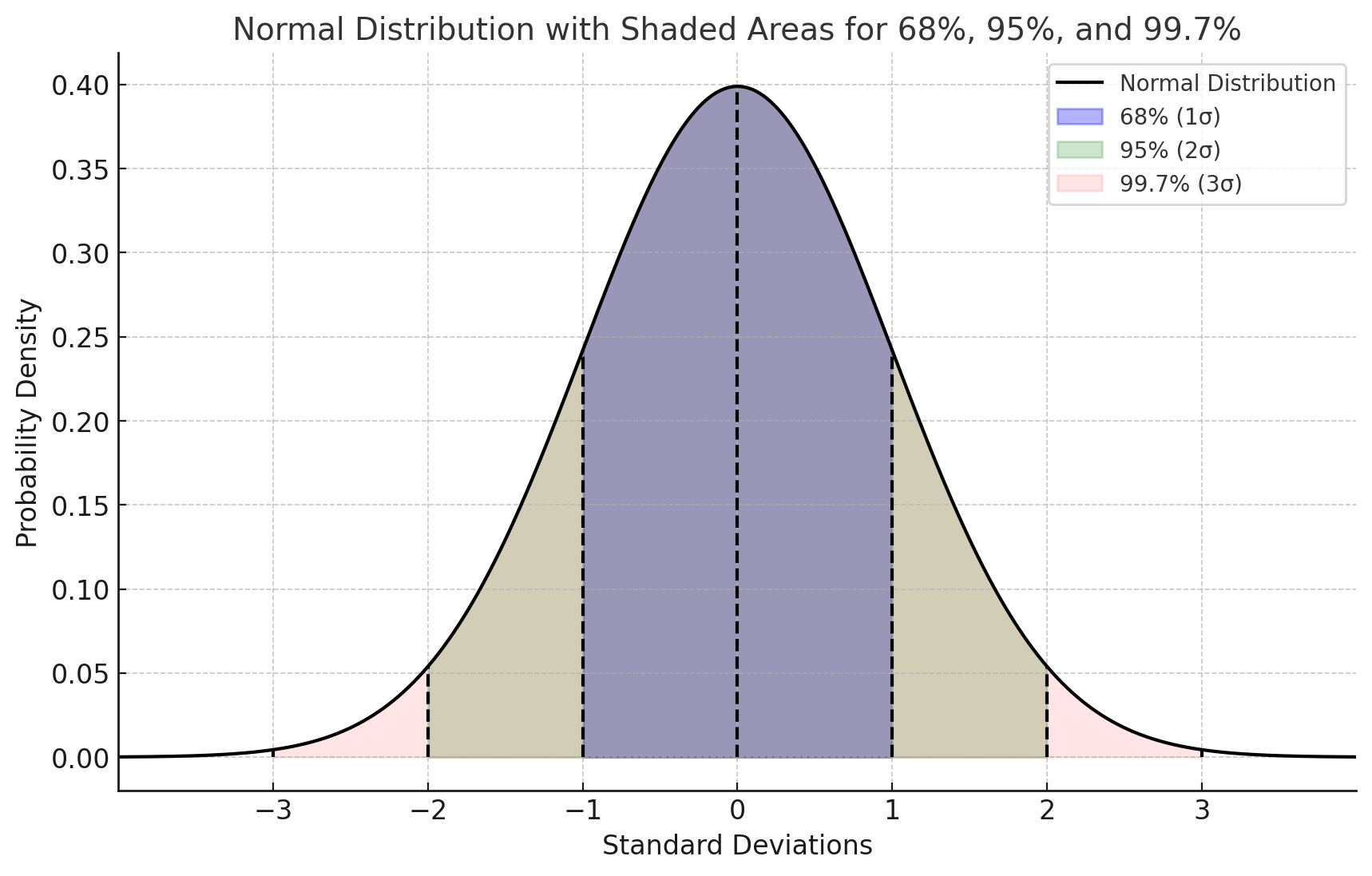
In a normally distributed dataset:

• 68% of data falls within \(\mu \pm \sigma\)

• 95% within \(\mu \pm 2\sigma\)

• 99.7% within \(\mu \pm 3\sigma\)

Histograms and Kernel Density Estimation (KDE)

Histograms:

• Visualize data distribution by binning values and counting frequencies.

• If data is Gaussian, the histogram approximates a bell curve.

KDE:

• A non-parametric way to estimate the PDF by smoothing individual data points with a kernel function.

• The KDE for a dataset \(X = \{x_1, x_2, \ldots, x_n\}\) is given by:

\[\hat{f}(x) = \frac{1}{nh} \sum_{i=1}^{n} K\left(\frac{x - x_i}{h}\right)\]

where:

• \(K\) is the kernel function (often Gaussian)

• \(h\) is the bandwidth (smoothing parameter)

Combined Use of Histograms and KDE

• Histograms offer a discrete, binned view of the data.

• KDE provides a smooth, continuous estimate of the underlying distribution.

• Together, they effectively illustrate how well the data aligns with the Gaussian assumption, highlighting any deviations from normality.

Pearson Correlation Coefficient

The Pearson correlation coefficient, often denoted as \(r\), is a measure of the linear relationship between two variables. It quantifies the degree to which a change in one variable is associated with a change in another variable. The Pearson correlation ranges from \(-1\) to \(1\), where:

• \(r = 1\) indicates a perfect positive linear relationship.

• \(r = -1\) indicates a perfect negative linear relationship.

• \(r = 0\) indicates no linear relationship.

The Pearson correlation coefficient between two variables \(X\) and \(Y\) is defined as:

\[r_{XY} = \frac{\text{Cov}(X, Y)}{\sigma_X \sigma_Y}\]

where:

• \(\text{Cov}(X, Y)\) is the covariance of \(X\) and \(Y\).

• \(\sigma_X\) is the standard deviation of \(X\).

• \(\sigma_Y\) is the standard deviation of \(Y\).

Covariance measures how much two variables change together. It is defined as:

\[\text{Cov}(X, Y) = \frac{1}{n} \sum_{i=1}^{n} (X_i - \mu_X)(Y_i - \mu_Y)\]

where:

• \(n\) is the number of data points.

• \(X_i\) and \(Y_i\) are the individual data points.

• \(\mu_X\) and \(\mu_Y\) are the means of \(X\) and \(Y\).

The standard deviation measures the dispersion or spread of a set of values. For a variable \(X\), the standard deviation \(\sigma_X\) is:

\[\sigma_X = \sqrt{\frac{1}{n} \sum_{i=1}^{n} (X_i - \mu_X)^2}\]

Substituting the covariance and standard deviation into the Pearson correlation formula:

\[r_{XY} = \frac{\sum_{i=1}^{n} (X_i - \mu_X)(Y_i - \mu_Y)}{\sqrt{\sum_{i=1}^{n} (X_i - \mu_X)^2} \sqrt{\sum_{i=1}^{n} (Y_i - \mu_Y)^2}}\]

This formula normalizes the covariance by the product of the standard deviations of the two variables, resulting in a dimensionless coefficient that indicates the strength and direction of the linear relationship between \(X\) and \(Y\).

• \(r > 0\): Positive correlation. As \(X\) increases, \(Y\) tends to increase.

• \(r < 0\): Negative correlation. As \(X\) increases, \(Y\) tends to decrease.

• \(r = 0\): No linear correlation. There is no consistent linear relationship between \(X\) and \(Y\).

The closer the value of \(r\) is to \(\pm 1\), the stronger the linear relationship between the two variables.

Box-Cox Transformation

The Box-Cox transformation is a powerful technique for stabilizing variance and making data more closely follow a normal distribution. Developed by statisticians George Box and David Cox in 1964, the transformation is particularly useful in linear regression models where assumptions of normality and homoscedasticity are necessary. This document provides an accessible overview of the theoretical concepts underlying the Box-Cox transformation.

Many statistical methods assume that data is normally distributed and that the variance remains constant across observations (homoscedasticity). However, real-world data often violates these assumptions, especially when dealing with positive-only, skewed distributions (e.g., income, expenditure, biological measurements). The Box-Cox transformation is a family of power transformations designed to address these issues by “normalizing” the data and stabilizing variance.

Mathematical Definition

The Box-Cox transformation is defined as follows:

\[\begin{split}y(\lambda) = \begin{cases} \frac{y^{\lambda} - 1}{\lambda}, & \text{if } \lambda \neq 0 \\ \ln(y), & \text{if } \lambda = 0 \end{cases}\end{split}\]

Here:

• \(y(\lambda)\) is the transformed variable,

• \(y\) is the original variable (positive and continuous),

• \(\lambda\) is the transformation parameter.

When \(\lambda = 0\), the transformation becomes a natural logarithm, effectively a special case of the Box-Cox transformation.

Interpretation of the Lambda Parameter

The value of \(\lambda\) determines the shape of the transformation:

• \(\lambda = 1\): The transformation does nothing; the data remains unchanged.

• \(\lambda = 0.5\): A square-root transformation.

• \(\lambda = 0\): A logarithmic transformation.

• \(\lambda < 0\): An inverse transformation, which is often helpful when working with highly skewed data.

Selecting the optimal value of \(\lambda\) to achieve approximate normality or homoscedasticity is typically done using maximum likelihood estimation (MLE), where the goal is to find the value of \(\lambda\) that maximizes the likelihood of observing the transformed data under a normal distribution.

Properties and Benefits

The Box-Cox transformation has two key properties:

1. Variance Stabilization: By choosing an appropriate \(\lambda\), the variance of \(y(\lambda)\) can be made more constant across levels of \(y\). This is particularly useful in regression analysis, as homoscedasticity is often a critical assumption.

2. Normalization: The transformation makes the distribution of \(y(\lambda)\) closer to normality. This allows statistical techniques that assume normality to be more applicable to real-world, skewed data.

Likelihood Function

The likelihood function for the Box-Cox transformation is derived from the assumption that the transformed data follows a normal distribution. For a dataset with observations \(y_i\), the likelihood function is given by:

\[L(\lambda) = -\frac{n}{2} \ln (s^2) + (\lambda - 1) \sum_{i=1}^{n} \ln(y_i),\]

where:

• \(n\) is the number of observations,

• \(s^2\) is the sample variance of the transformed data.

Maximizing this likelihood function provides the MLE for \(\lambda\), which can be estimated using iterative methods.

Practical Considerations

In practice, implementing the Box-Cox transformation requires a few considerations:

• Positive-Only Data: The transformation is only defined for positive values. For datasets with zero or negative values, a constant can be added to make all observations positive before applying the transformation.

• Interpretability: The transformed data may lose interpretability in its original scale. For some applications, this trade-off is justified to meet model assumptions.

• Inverse Transformation: If interpretability is a concern, the inverse of the Box-Cox transformation can be applied to transform results back to the original scale.

Applications in Modeling

In regression modeling, the Box-Cox transformation can improve both the accuracy and validity of predictions. For example, in Ordinary Least Squares (OLS) regression, the transformation reduces heteroscedasticity and normalizes residuals, leading to more reliable parameter estimates. Similarly, in time series analysis, the Box-Cox transformation can stabilize variance, making models such as ARIMA more effective.

The Box-Cox transformation is a flexible and powerful technique for addressing non-normality and heteroscedasticity in data. By choosing an appropriate \(\lambda\), practitioners can transform data to better meet the assumptions of various statistical methods, enhancing the reliability of their models and inferences.

Confidence Intervals for Lambda

In practice, it is often helpful to assess the stability of the estimated transformation parameter \(\lambda\) by constructing a confidence interval (CI). The CI provides a range of values within which the true value of \(\lambda\) is likely to fall, offering insights into the sensitivity of the transformation.

To construct a confidence interval for \(\lambda\), the following approach can be used:

1. Alpha Level: Select an alpha level, commonly 0.05, for a 95% confidence interval, or adjust as needed. The alpha level represents the probability of observing a value outside this interval if the estimate were repeated multiple times.

2. Profile Likelihood Method: One approach is to use the profile likelihood method, where a range of \(\lambda\) values are tested, and those with likelihoods close to the maximum likelihood estimate (MLE) are retained within the interval. The confidence interval is defined as the set of \(\lambda\) values for which the likelihood ratio statistic:

\[\text{LR}(\lambda) = 2 \left( L(\hat{\lambda}) - L(\lambda) \right)\]

is less than the chi-square value at the chosen confidence level (e.g., 3.84 for a 95% CI with one degree of freedom).

3. Interpretation: A narrow CI around \(\lambda\) suggests that the transformation is relatively stable, while a wide interval might indicate sensitivity, signaling that the data may benefit from an alternative transformation or modeling approach.

These confidence intervals provide a more robust understanding of the transformation’s impact, as well as the degree of transformation needed to meet model assumptions.

The Yeo-Johnson Transformation

For a feature \(y\), the Yeo-Johnson transformation \(Y\) is defined as:

\[\begin{split}Y = \begin{cases} \frac{((y + 1)^{\lambda} - 1)}{\lambda} & \text{if } y \geq 0, \lambda \neq 0 \\ \ln(y + 1) & \text{if } y \geq 0, \lambda = 0 \\ -\frac{((-y + 1)^{2 - \lambda} - 1)}{2 - \lambda} & \text{if } y < 0, \lambda \neq 2 \\ -\ln(-y + 1) & \text{if } y < 0, \lambda = 2 \end{cases}\end{split}\]

Breakdown of the Conditions

1. For Positive Values of \(y\) (\(y \geq 0\)):

   • When \(\lambda \neq 0\): The transformation behaves similarly to the Box-Cox transformation with \((y + 1)^{\lambda}\).

   • When \(\lambda = 0\): The transformation simplifies to the natural log, \(\ln(y + 1)\).

2. For Negative Values of \(y\) (\(y < 0\)):

   • When \(\lambda \neq 2\): A reflected transformation is applied, \(-(−y + 1)^{2 - \lambda}\), to manage negative values smoothly.

   • When \(\lambda = 2\): The transformation simplifies to \(- \ln(-y + 1)\), making it suitable for negative inputs while preserving continuity.

Why It Works

The Yeo-Johnson transformation adjusts data to make it more normally distributed. By allowing transformations for both positive and negative values, it offers flexibility across various distributions. The parameter \(\lambda\) is typically optimized to best approximate normality.

When to Use It

Yeo-Johnson is particularly useful for datasets containing zero or negative values. It’s often effective for linear models that assume normally distributed data, making it a robust alternative when Box-Cox cannot be applied.

Median and IQR Scaling

RobustScaler in scikit-learn is a scaling method that reduces the impact of outliers in your data by using the median and interquartile range (IQR) instead of the mean and standard deviation, which are more sensitive to extreme values. Here’s a mathematical breakdown of how it works:

Centering Data Using the Median

The formula for scaling each feature \(x\) in the dataset using RobustScaler is:

\[x_{\text{scaled}} = \frac{x - \text{Median}(x)}{\text{IQR}(x)}\]

where:

• \(\text{Median}(x)\) is the median of the feature \(x\).

• \(\text{IQR}(x) = Q_3 - Q_1\), the interquartile range, is the difference between the 75th percentile (\(Q_3\)) and the 25th percentile (\(Q_1\)) of the feature. This range represents the spread of the middle 50% of values, which is less sensitive to extreme values than the total range.

Explanation of Each Component

• Median (\(\text{Median}(x)\)): This is the 50th percentile, or the central value of the feature. It acts as the “center” of the data, but unlike the mean, it is robust to outliers.

• Interquartile Range (IQR): By dividing by the IQR, the RobustScaler standardizes the spread of the data based on the range of the middle 50% of values, making it less influenced by extreme values. Essentially, the values are scaled to fall within a range close to -1 to 1 for the majority of samples.

Example Calculation

Suppose you have a feature \(x = [1, 2, 3, 4, 5, 100]\). Here’s how the scaling would work:

1. Calculate the Median:

   \[\text{Median}(x) = 3.5\]

2. Calculate the Interquartile Range (IQR):

   • First, find \(Q_1\) (25th percentile) and \(Q_3\) (75th percentile): - \(Q_1 = 2\), \(Q_3 = 5\)

   • Then, \(\text{IQR}(x) = Q_3 - Q_1 = 5 - 2 = 3\)

3. Apply the Scaling Formula:

   • For each \(x\) value, subtract the median and divide by the IQR:

   \[x_{\text{scaled}} = \frac{x - 3.5}{3}\]

This results in values that are centered around 0 and scaled according to the interquartile range, rather than the full range or mean and standard deviation. For our example, the outlier (100) will be downscaled effectively, reducing its influence on the data’s range and making the scaling robust to such outliers.

The RobustScaler is particularly useful when dealing with data with significant outliers, as it centers the data around the median and scales according to the IQR, allowing for better handling of extreme values than traditional standardization methods.

Logit Transformation

The logit transformation is used to map values from the range \((0, 1)\) to the entire real number line \((-\infty, +\infty)\). It is defined mathematically as:

\[\text{logit}(p) = \ln\left(\frac{p}{1 - p}\right)\]

where \(p\) is a value in the range \((0, 1)\). In other words, for each value \(p\), the transformation is calculated by taking the natural logarithm of the odds \(p / (1 - p)\).

Purpose and Assumptions

The logit function is particularly useful in scenarios where data is constrained between 0 and 1, such as probabilities or proportions. However, to apply this transformation, all values must strictly lie within the open interval \((0, 1)\). Values equal to 0 or 1 result in undefined values \((-\infty, +\infty\) respectively) since the logarithm of zero is undefined.

In the code implementation, a ValueError is raised if any values in the target feature fall outside the interval \((0, 1)\). If your data does not meet this condition, consider applying a Min-Max scaling first to transform the data to the appropriate range.

Example

If \(p = 0.5\), then:

\[\text{logit}(0.5) = \ln\left(\frac{0.5}{1 - 0.5}\right) = \ln(1) = 0\]

Partial Dependence Foundations

Let \(\mathbf{X}\) represent the complete set of input features for a machine learning model, where \(\mathbf{X} = \{X_1, X_2, \dots, X_p\}\). Suppose we’re particularly interested in a subset of these features, denoted by \(\mathbf{X}_S\). The complementary set, \(\mathbf{X}_C\), contains all the features in \(\mathbf{X}\) that are not in \(\mathbf{X}_S\). Mathematically, this relationship is expressed as:

\[\mathbf{X}_C = \mathbf{X} \setminus \mathbf{X}_S\]

where \(\mathbf{X}_C\) is the set of features in \(\mathbf{X}\) after removing the features in \(\mathbf{X}_S\).

Partial Dependence Plots (PDPs) are used to illustrate the effect of the features in \(\mathbf{X}_S\) on the model’s predictions, while averaging out the influence of the features in \(\mathbf{X}_C\). This is mathematically defined as:

\[\begin{split}\begin{align*} \text{PD}_{\mathbf{X}_S}(x_S) &= \mathbb{E}_{\mathbf{X}_C} \left[ f(x_S, \mathbf{X}_C) \right] \\ &= \int f(x_S, x_C) \, p(x_C) \, dx_C \\ &= \int \left( \int f(x_S, x_C) \, p(x_C \mid x_S) \, dx_C \right) p(x_S) \, dx_S \end{align*}\end{split}\]

where:

• \(\mathbb{E}_{\mathbf{X}_C} \left[ \cdot \right]\) indicates that we are taking the expected value over the possible values of the features in the set \(\mathbf{X}_C\).

• \(p(x_C)\) represents the probability density function of the features in \(\mathbf{X}_C\).

This operation effectively summarizes the model’s output over all potential values of the complementary features, providing a clear view of how the features in \(\mathbf{X}_S\) alone impact the model’s predictions.

2D Partial Dependence Plots

Consider a trained machine learning model 2D Partial Dependence Plots\(f(\mathbf{X})\), where \(\mathbf{X} = (X_1, X_2, \dots, X_p)\) represents the vector of input features. The partial dependence of the predicted response \(\hat{y}\) on a single feature \(X_j\) is defined as:

\[\text{PD}(X_j) = \frac{1}{n} \sum_{i=1}^{n} f(X_j, \mathbf{X}_{C_i})\]

where:

• \(X_j\) is the feature of interest.

• \(\mathbf{X}_{C_i}\) represents the complement set of \(X_j\), meaning the remaining features in \(\mathbf{X}\) not included in \(X_j\) for the \(i\)-th instance.

• \(n\) is the number of observations in the dataset.

For two features, \(X_j\) and \(X_k\), the partial dependence is given by:

\[\text{PD}(X_j, X_k) = \frac{1}{n} \sum_{i=1}^{n} f(X_j, X_k, \mathbf{X}_{C_i})\]

This results in a 2D surface plot (or contour plot) that shows how the predicted outcome changes as the values of \(X_j\) and \(X_k\) vary, while the effects of the other features are averaged out.

• Single Feature PDP: When plotting \(\text{PD}(X_j)\), the result is a 2D line plot showing the marginal effect of feature \(X_j\) on the predicted outcome, averaged over all possible values of the other features.

• Two Features PDP: When plotting \(\text{PD}(X_j, X_k)\), the result is a 3D surface plot (or a contour plot) that shows the combined marginal effect of \(X_j\) and \(X_k\) on the predicted outcome. The surface represents the expected value of the prediction as \(X_j\) and \(X_k\) vary, while all other features are averaged out.

3D Partial Dependence Plots

For a more comprehensive analysis, especially when exploring interactions between two features, 3D Partial Dependence Plots are invaluable. The partial dependence function for two features in a 3D context is:

\[\text{PD}(X_j, X_k) = \frac{1}{n} \sum_{i=1}^{n} f(X_j, X_k, \mathbf{X}_{C_i})\]

Here, the function \(f(X_j, X_k, \mathbf{X}_{C_i})\) is evaluated across a grid of values for \(X_j\) and \(X_k\). The resulting 3D surface plot represents how the model’s prediction changes over the joint range of these two features.

The 3D plot offers a more intuitive visualization of feature interactions compared to 2D contour plots, allowing for a better understanding of the combined effects of features on the model’s predictions. The surface plot is particularly useful when you need to capture complex relationships that might not be apparent in 2D.

• Feature Interaction Visualization: The 3D PDP provides a comprehensive view of the interaction between two features. The resulting surface plot allows for the visualization of how the model’s output changes when the values of two features are varied simultaneously, making it easier to understand complex interactions.

• Enhanced Interpretation: 3D PDPs offer enhanced interpretability in scenarios where feature interactions are not linear or where the effect of one feature depends on the value of another. The 3D visualization makes these dependencies more apparent.