Gaussian Assumption for Normality

The Gaussian (normal) distribution is a key assumption in many statistical methods. It is mathematically represented by the probability density function (PDF):

\[f(x) = \frac{1}{\sqrt{2\pi\sigma^2}} \exp\left(-\frac{(x-\mu)^2}{2\sigma^2}\right)\]

where:

• \(\mu\) is the mean

• \(\sigma^2\) is the variance

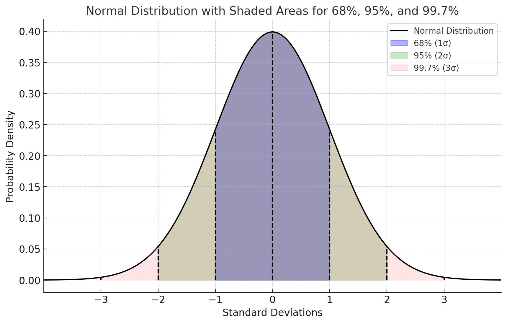
In a normally distributed dataset:

• 68% of data falls within \(\mu \pm \sigma\)

• 95% within \(\mu \pm 2\sigma\)

• 99.7% within \(\mu \pm 3\sigma\)

Histograms and Kernel Density Estimation (KDE)

Histograms:

• Visualize data distribution by binning values and counting frequencies.

• If data is Gaussian, the histogram approximates a bell curve.

KDE:

• A non-parametric way to estimate the PDF by smoothing individual data points with a kernel function.

• The KDE for a dataset \(X = \{x_1, x_2, \ldots, x_n\}\) is given by:

\[\hat{f}(x) = \frac{1}{nh} \sum_{i=1}^{n} K\left(\frac{x - x_i}{h}\right)\]

where:

• \(K\) is the kernel function (often Gaussian)

• \(h\) is the bandwidth (smoothing parameter)

Combined Use of Histograms and KDE

• Histograms offer a discrete, binned view of the data.

• KDE provides a smooth, continuous estimate of the underlying distribution.

• Together, they effectively illustrate how well the data aligns with the Gaussian assumption, highlighting any deviations from normality.

Pearson Correlation Coefficient

The Pearson correlation coefficient, often denoted as \(r\), is a measure of the linear relationship between two variables. It quantifies the degree to which a change in one variable is associated with a change in another variable. The Pearson correlation ranges from \(-1\) to \(1\), where:

• \(r = 1\) indicates a perfect positive linear relationship.

• \(r = -1\) indicates a perfect negative linear relationship.

• \(r = 0\) indicates no linear relationship.

The Pearson correlation coefficient between two variables \(X\) and \(Y\) is defined as:

\[r_{XY} = \frac{\text{Cov}(X, Y)}{\sigma_X \sigma_Y}\]

where:

• \(\text{Cov}(X, Y)\) is the covariance of \(X\) and \(Y\).

• \(\sigma_X\) is the standard deviation of \(X\).

• \(\sigma_Y\) is the standard deviation of \(Y\).

Covariance measures how much two variables change together. It is defined as:

\[\text{Cov}(X, Y) = \frac{1}{n} \sum_{i=1}^{n} (X_i - \mu_X)(Y_i - \mu_Y)\]

where:

• \(n\) is the number of data points.

• \(X_i\) and \(Y_i\) are the individual data points.

• \(\mu_X\) and \(\mu_Y\) are the means of \(X\) and \(Y\).

The standard deviation measures the dispersion or spread of a set of values. For a variable \(X\), the standard deviation \(\sigma_X\) is:

\[\sigma_X = \sqrt{\frac{1}{n} \sum_{i=1}^{n} (X_i - \mu_X)^2}\]

Substituting the covariance and standard deviation into the Pearson correlation formula:

\[r_{XY} = \frac{\sum_{i=1}^{n} (X_i - \mu_X)(Y_i - \mu_Y)}{\sqrt{\sum_{i=1}^{n} (X_i - \mu_X)^2} \sqrt{\sum_{i=1}^{n} (Y_i - \mu_Y)^2}}\]

This formula normalizes the covariance by the product of the standard deviations of the two variables, resulting in a dimensionless coefficient that indicates the strength and direction of the linear relationship between \(X\) and \(Y\).

• \(r > 0\): Positive correlation. As \(X\) increases, \(Y\) tends to increase.

• \(r < 0\): Negative correlation. As \(X\) increases, \(Y\) tends to decrease.

• \(r = 0\): No linear correlation. There is no consistent linear relationship between \(X\) and \(Y\).

The closer the value of \(r\) is to \(\pm 1\), the stronger the linear relationship between the two variables.

Box-Cox Transformation

The Box-Cox transformation is a powerful technique for stabilizing variance and making data more closely follow a normal distribution. Developed by statisticians George Box and David Cox in 1964, the transformation is particularly useful in linear regression models where assumptions of normality and homoscedasticity are necessary. This document provides an accessible overview of the theoretical concepts underlying the Box-Cox transformation.

Many statistical methods assume that data is normally distributed and that the variance remains constant across observations (homoscedasticity). However, real-world data often violates these assumptions, especially when dealing with positive-only, skewed distributions (e.g., income, expenditure, biological measurements). The Box-Cox transformation is a family of power transformations designed to address these issues by “normalizing” the data and stabilizing variance.

Mathematical Definition

The Box-Cox transformation is defined as follows:

\[\begin{split}y(\lambda) = \begin{cases} \frac{y^{\lambda} - 1}{\lambda}, & \text{if } \lambda \neq 0 \\ \ln(y), & \text{if } \lambda = 0 \end{cases}\end{split}\]

Here:

• \(y(\lambda)\) is the transformed variable,

• \(y\) is the original variable (positive and continuous),

• \(\lambda\) is the transformation parameter.

When \(\lambda = 0\), the transformation becomes a natural logarithm, effectively a special case of the Box-Cox transformation.

Interpretation of the Lambda Parameter

The value of \(\lambda\) determines the shape of the transformation:

• \(\lambda = 1\): The transformation does nothing; the data remains unchanged.

• \(\lambda = 0.5\): A square-root transformation.

• \(\lambda = 0\): A logarithmic transformation.

• \(\lambda < 0\): An inverse transformation, which is often helpful when working with highly skewed data.

Selecting the optimal value of \(\lambda\) to achieve approximate normality or homoscedasticity is typically done using maximum likelihood estimation (MLE), where the goal is to find the value of \(\lambda\) that maximizes the likelihood of observing the transformed data under a normal distribution.

Properties and Benefits

The Box-Cox transformation has two key properties:

1. Variance Stabilization: By choosing an appropriate \(\lambda\), the variance of \(y(\lambda)\) can be made more constant across levels of \(y\). This is particularly useful in regression analysis, as homoscedasticity is often a critical assumption.

2. Normalization: The transformation makes the distribution of \(y(\lambda)\) closer to normality. This allows statistical techniques that assume normality to be more applicable to real-world, skewed data.

Likelihood Function

The likelihood function for the Box-Cox transformation is derived from the assumption that the transformed data follows a normal distribution. For a dataset with observations \(y_i\), the likelihood function is given by:

\[L(\lambda) = -\frac{n}{2} \ln (s^2) + (\lambda - 1) \sum_{i=1}^{n} \ln(y_i),\]

where:

• \(n\) is the number of observations,

• \(s^2\) is the sample variance of the transformed data.

Maximizing this likelihood function provides the MLE for \(\lambda\), which can be estimated using iterative methods.

Practical Considerations

In practice, implementing the Box-Cox transformation requires a few considerations:

• Positive-Only Data: The transformation is only defined for positive values. For datasets with zero or negative values, a constant can be added to make all observations positive before applying the transformation.

• Interpretability: The transformed data may lose interpretability in its original scale. For some applications, this trade-off is justified to meet model assumptions.

• Inverse Transformation: If interpretability is a concern, the inverse of the Box-Cox transformation can be applied to transform results back to the original scale.

Applications in Modeling

In regression modeling, the Box-Cox transformation can improve both the accuracy and validity of predictions. For example, in Ordinary Least Squares (OLS) regression, the transformation reduces heteroscedasticity and normalizes residuals, leading to more reliable parameter estimates. Similarly, in time series analysis, the Box-Cox transformation can stabilize variance, making models such as ARIMA more effective.

The Box-Cox transformation is a flexible and powerful technique for addressing non-normality and heteroscedasticity in data. By choosing an appropriate \(\lambda\), practitioners can transform data to better meet the assumptions of various statistical methods, enhancing the reliability of their models and inferences.

Confidence Intervals for Lambda

In practice, it is often helpful to assess the stability of the estimated transformation parameter \(\lambda\) by constructing a confidence interval (CI). The CI provides a range of values within which the true value of \(\lambda\) is likely to fall, offering insights into the sensitivity of the transformation.

To construct a confidence interval for \(\lambda\), the following approach can be used:

1. Alpha Level: Select an alpha level, commonly 0.05, for a 95% confidence interval, or adjust as needed. The alpha level represents the probability of observing a value outside this interval if the estimate were repeated multiple times.

2. Profile Likelihood Method: One approach is to use the profile likelihood method, where a range of \(\lambda\) values are tested, and those with likelihoods close to the maximum likelihood estimate (MLE) are retained within the interval. The confidence interval is defined as the set of \(\lambda\) values for which the likelihood ratio statistic:

\[\text{LR}(\lambda) = 2 \left( L(\hat{\lambda}) - L(\lambda) \right)\]

is less than the chi-square value at the chosen confidence level (e.g., 3.84 for a 95% CI with one degree of freedom).

3. Interpretation: A narrow CI around \(\lambda\) suggests that the transformation is relatively stable, while a wide interval might indicate sensitivity, signaling that the data may benefit from an alternative transformation or modeling approach.

These confidence intervals provide a more robust understanding of the transformation’s impact, as well as the degree of transformation needed to meet model assumptions.

The Yeo-Johnson Transformation

For a feature \(y\), the Yeo-Johnson transformation \(Y\) is defined as:

\[\begin{split}Y = \begin{cases} \frac{((y + 1)^{\lambda} - 1)}{\lambda} & \text{if } y \geq 0, \lambda \neq 0 \\ \ln(y + 1) & \text{if } y \geq 0, \lambda = 0 \\ -\frac{((-y + 1)^{2 - \lambda} - 1)}{2 - \lambda} & \text{if } y < 0, \lambda \neq 2 \\ -\ln(-y + 1) & \text{if } y < 0, \lambda = 2 \end{cases}\end{split}\]

Breakdown of the Conditions

1. For Positive Values of \(y\) (\(y \geq 0\)):

   • When \(\lambda \neq 0\): The transformation behaves similarly to the Box-Cox transformation with \((y + 1)^{\lambda}\).

   • When \(\lambda = 0\): The transformation simplifies to the natural log, \(\ln(y + 1)\).

2. For Negative Values of \(y\) (\(y < 0\)):

   • When \(\lambda \neq 2\): A reflected transformation is applied, \(-(−y + 1)^{2 - \lambda}\), to manage negative values smoothly.

   • When \(\lambda = 2\): The transformation simplifies to \(- \ln(-y + 1)\), making it suitable for negative inputs while preserving continuity.

Why It Works

The Yeo-Johnson transformation adjusts data to make it more normally distributed. By allowing transformations for both positive and negative values, it offers flexibility across various distributions. The parameter \(\lambda\) is typically optimized to best approximate normality.

When to Use It

Yeo-Johnson is particularly useful for datasets containing zero or negative values. It’s often effective for linear models that assume normally distributed data, making it a robust alternative when Box-Cox cannot be applied.

Median and IQR Scaling

RobustScaler in scikit-learn is a scaling method that reduces the impact of outliers in your data by using the median and interquartile range (IQR) instead of the mean and standard deviation, which are more sensitive to extreme values. Here’s a mathematical breakdown of how it works:

Centering Data Using the Median

The formula for scaling each feature \(x\) in the dataset using RobustScaler is:

\[x_{\text{scaled}} = \frac{x - \text{Median}(x)}{\text{IQR}(x)}\]

where:

• \(\text{Median}(x)\) is the median of the feature \(x\).

• \(\text{IQR}(x) = Q_3 - Q_1\), the interquartile range, is the difference between the 75th percentile (\(Q_3\)) and the 25th percentile (\(Q_1\)) of the feature. This range represents the spread of the middle 50% of values, which is less sensitive to extreme values than the total range.

Explanation of Each Component

• Median (\(\text{Median}(x)\)): This is the 50th percentile, or the central value of the feature. It acts as the “center” of the data, but unlike the mean, it is robust to outliers.

• Interquartile Range (IQR): By dividing by the IQR, the RobustScaler standardizes the spread of the data based on the range of the middle 50% of values, making it less influenced by extreme values. Essentially, the values are scaled to fall within a range close to -1 to 1 for the majority of samples.

Example Calculation

Suppose you have a feature \(x = [1, 2, 3, 4, 5, 100]\). Here’s how the scaling would work:

1. Calculate the Median:

   \[\text{Median}(x) = 3.5\]

2. Calculate the Interquartile Range (IQR):

   • First, find \(Q_1\) (25th percentile) and \(Q_3\) (75th percentile): - \(Q_1 = 2\), \(Q_3 = 5\)

   • Then, \(\text{IQR}(x) = Q_3 - Q_1 = 5 - 2 = 3\)

3. Apply the Scaling Formula:

   • For each \(x\) value, subtract the median and divide by the IQR:

   \[x_{\text{scaled}} = \frac{x - 3.5}{3}\]

This results in values that are centered around 0 and scaled according to the interquartile range, rather than the full range or mean and standard deviation. For our example, the outlier (100) will be downscaled effectively, reducing its influence on the data’s range and making the scaling robust to such outliers.

The RobustScaler is particularly useful when dealing with data with significant outliers, as it centers the data around the median and scales according to the IQR, allowing for better handling of extreme values than traditional standardization methods.

Logit Transformation

The logit transformation is used to map values from the range \((0, 1)\) to the entire real number line \((-\infty, +\infty)\). It is defined mathematically as:

\[\text{logit}(p) = \ln\left(\frac{p}{1 - p}\right)\]

where \(p\) is a value in the range \((0, 1)\). In other words, for each value \(p\), the transformation is calculated by taking the natural logarithm of the odds \(p / (1 - p)\).

Purpose and Assumptions

The logit function is particularly useful in scenarios where data is constrained between 0 and 1, such as probabilities or proportions. However, to apply this transformation, all values must strictly lie within the open interval \((0, 1)\). Values equal to 0 or 1 result in undefined values \((-\infty, +\infty\) respectively) since the logarithm of zero is undefined.

In the code implementation, a ValueError is raised if any values in the target feature fall outside the interval \((0, 1)\). If your data does not meet this condition, consider applying a Min-Max scaling first to transform the data to the appropriate range.

Example

If \(p = 0.5\), then:

\[\text{logit}(0.5) = \ln\left(\frac{0.5}{1 - 0.5}\right) = \ln(1) = 0\]

Parameter Estimation for Density Models and Distribution GOF Plots

When fitting parametric probability density functions to data, the key task is to estimate the unknown parameters of the assumed distribution. In plot_distributions and distribution_gof_plots, this estimation step is required whenever a parametric density (e.g., Normal, Lognormal, Gamma) is overlaid on the empirical distribution.

Two classical estimation frameworks are commonly used for this purpose:

• Method of Moments (MoM)

• Maximum Likelihood Estimation (MLE)

Both approaches seek to infer distributional parameters from observed data, but they do so using fundamentally different principles.

Method of Moments (MoM)

The Method of Moments estimates distribution parameters by equating theoretical moments of a probability distribution to the corresponding sample moments computed from the data.

Let \(X_1, X_2, \dots, X_n\) be a random sample drawn from a distribution with parameter vector \(\theta\). The \(k^{th}\) theoretical moment is:

\[\mu_k(\theta) = \mathbb{E}[X^k]\]

The corresponding sample moment is:

\[\hat{\mu}_k = \frac{1}{n} \sum_{i=1}^{n} X_i^k\]

The Method of Moments estimator \(\hat{\theta}_{\text{MoM}}\) is obtained by solving the system:

\[\mu_k(\theta) = \hat{\mu}_k \quad \text{for } k = 1, \dots, p\]

where \(p\) is the number of parameters in the distribution.

Example: Normal Distribution

For a Normal distribution \(\mathcal{N}(\mu, \sigma^2)\):

• First theoretical moment: \(\mathbb{E}[X] = \mu\)

• Second central moment: \(\mathbb{E}[(X - \mu)^2] = \sigma^2\)

Equating moments yields:

\[\hat{\mu}_{\text{MoM}} = \bar{X}, \quad \hat{\sigma}^2_{\text{MoM}} = \frac{1}{n} \sum_{i=1}^{n} (X_i - \bar{X})^2\]

Characteristics of MoM

• Computationally simple and fast

• Closed-form solutions for many distributions

• Does not require specifying a likelihood function

• Can be inefficient or biased for small samples

• Does not optimize a global objective

Method of Moments is often used as a baseline or initialization strategy, especially when likelihood optimization is unstable.

Maximum Likelihood Estimation (MLE)

Maximum Likelihood Estimation estimates parameters by maximizing the probability of observing the given data under the assumed distribution.

Let \(f(x \mid \theta)\) be the probability density function of a distribution with parameter vector \(\theta\). The likelihood function for an i.i.d. sample is:

\[\mathcal{L}(\theta \mid X) = \prod_{i=1}^{n} f(X_i \mid \theta)\]

It is more convenient to work with the log-likelihood:

\[\ell(\theta) = \sum_{i=1}^{n} \log f(X_i \mid \theta)\]

The MLE estimator \(\hat{\theta}_{\text{MLE}}\) is defined as:

\[\hat{\theta}_{\text{MLE}} = \arg\max_{\theta} \; \ell(\theta)\]

Example: Normal Distribution

For \(X_i \sim \mathcal{N}(\mu, \sigma^2)\):

\[\ell(\mu, \sigma^2) = -\frac{n}{2} \log(2\pi\sigma^2) - \frac{1}{2\sigma^2} \sum_{i=1}^{n} (X_i - \mu)^2\]

Maximizing this expression yields:

\[\hat{\mu}_{\text{MLE}} = \bar{X}, \quad \hat{\sigma}^2_{\text{MLE}} = \frac{1}{n} \sum_{i=1}^{n} (X_i - \bar{X})^2\]

For the Normal distribution, MoM and MLE coincide. For many other distributions (e.g., Lognormal, Gamma), they differ substantially.

Characteristics of MLE

• Statistically efficient under correct model specification

• Asymptotically unbiased and consistent

• Naturally supports hypothesis testing and confidence intervals

• Requires numerical optimization for many distributions

• Sensitive to model misspecification and outliers

In practice, MLE is preferred when a well-justified parametric assumption is available and sample size is sufficient.

Relationship to Density Overlays

When plot_distributions overlays parametric densities on histograms or KDE curves, the following workflow is implicitly assumed:

1. A parametric family is selected (e.g., Normal, Lognormal).

2. Parameters are estimated using either:

   • Method of Moments, or

   • Maximum Likelihood Estimation.

3. The fitted probability density function is evaluated across the data range.

4. The resulting curve is plotted alongside the empirical distribution.

The choice between MoM and MLE affects the shape, scale, and tail behavior of the fitted density, and therefore influences how closely the parametric model aligns with the observed data.

Using multiple density overlays simultaneously allows visual comparison of different modeling assumptions and estimation strategies.

Empirical Cumulative Distribution Function: ECDF

The Empirical Cumulative Distribution Function (ECDF) provides a non-parametric estimate of the cumulative distribution function (CDF) of a random variable based directly on observed data. Unlike parametric approaches, the ECDF makes no assumptions about the underlying probability distribution and depends solely on the sample itself.

Definition

Let \(X_1, X_2, \dots, X_n\) be an independent and identically distributed sample drawn from an unknown distribution with true cumulative distribution function \(F(x)\).

The empirical cumulative distribution function \(\hat{F}_n(x)\) is defined as:

\[\hat{F}_n(x) = \frac{1}{n} \sum_{i=1}^{n} \mathbf{1}\{X_i \le x\}\]

where \(\mathbf{1}\{\cdot\}\) denotes the indicator function, which equals 1 if its argument is true and 0 otherwise.

Interpretation

For any real value \(x\), the ECDF \(\hat{F}_n(x)\) represents the proportion of observed data points less than or equal to \(x\). The ECDF is therefore a step function that:

• Starts at 0 and increases monotonically to 1

• Jumps upward by increments of \(1/n\) at each observed data point

• Is right-continuous with left limits

Each jump corresponds exactly to an observed value in the sample.

Statistical Properties

The ECDF possesses several important theoretical properties.

Consistency

By the Glivenko–Cantelli Theorem, the ECDF converges uniformly to the true CDF:

\[\sup_x \left| \hat{F}_n(x) - F(x) \right| \xrightarrow{a.s.} 0 \quad \text{as } n \to \infty\]

This guarantees that the ECDF is a strongly consistent estimator of the true distribution function.

Unbiasedness

For any fixed \(x\), the ECDF is an unbiased estimator of the true CDF:

\[\mathbb{E}[\hat{F}_n(x)] = F(x)\]

Variance

The variance of the ECDF at a fixed point \(x\) is given by:

\[\mathrm{Var}[\hat{F}_n(x)] = \frac{F(x)(1 - F(x))}{n}\]

This shows that uncertainty decreases at the standard parametric rate \(O(n^{-1})\).

Relationship to Order Statistics

Let \(X_{(1)} \le X_{(2)} \le \dots \le X_{(n)}\) denote the order statistics of the sample. The ECDF increases by exactly \(1/n\) at each order statistic:

\[\begin{split}\hat{F}_n(x) = \begin{cases} 0, & x < X_{(1)} \\ k/n, & X_{(k)} \le x < X_{(k+1)} \\ 1, & x \ge X_{(n)} \end{cases}\end{split}\]

This representation makes explicit the direct connection between the ECDF and the empirical quantile function.

Comparison with Histogram and KDE

The ECDF differs fundamentally from histogram- and kernel-based density estimates:

• Histograms depend on bin width and bin placement

• Kernel density estimates (KDEs) depend on bandwidth and kernel choice

• ECDFs require no tuning parameters and introduce no smoothing bias

As a result, ECDFs are particularly well suited for:

• Distributional diagnostics

• Model checking and goodness-of-fit assessment

• Comparing empirical and theoretical distributions

• Visualizing cumulative probability mass and tail behavior

Tail Behavior and Exceedance Functions

The ECDF naturally supports tail analysis through the empirical survival function (or exceedance function):

\[\hat{S}_n(x) = 1 - \hat{F}_n(x)\]

This representation is especially useful for analyzing upper-tail behavior, heavy-tailed distributions, and rare events, particularly when combined with logarithmic axis scaling.

Practical Considerations

• ECDFs are invariant to monotone transformations of the data ordering

• They remain interpretable under log or power transformations

• They provide exact cumulative probabilities at observed values

• They scale well computationally for large datasets

Because of these properties, ECDFs are a foundational tool in exploratory data analysis and serve as a robust complement to density-based visualizations.